Optimizing Heuristic Ranker
12 July 2026
So a while back, a few friends and I started a project called the Unofficial FCI Forums, a central platform for MMU FCI students to share information, which we launched around March 2026. We actually started building it two years ago, and... I would love to go through this entire journey, but that's a story for another day.
One key feature of the forum is its recommendation algorithm. Due to lack of resources, we started off with a simple heuristic ranker.

The heuristic ranker, denoted by , is defined as:
where is the post, is the net votes of the post, is the number of comments, is the age of the post in hours, and are weights, and is a bias term. The weights and biases are hyperparameters that we set almost arbitrarily.
Intuitively, the nominator is the "value" of a post and the denominator is the "decay" of that value over time, this is to ensure that newer posts are ranked higher than older posts (a key assumption we made for simplicity). Visually, this is how "decay" changes over time for different :
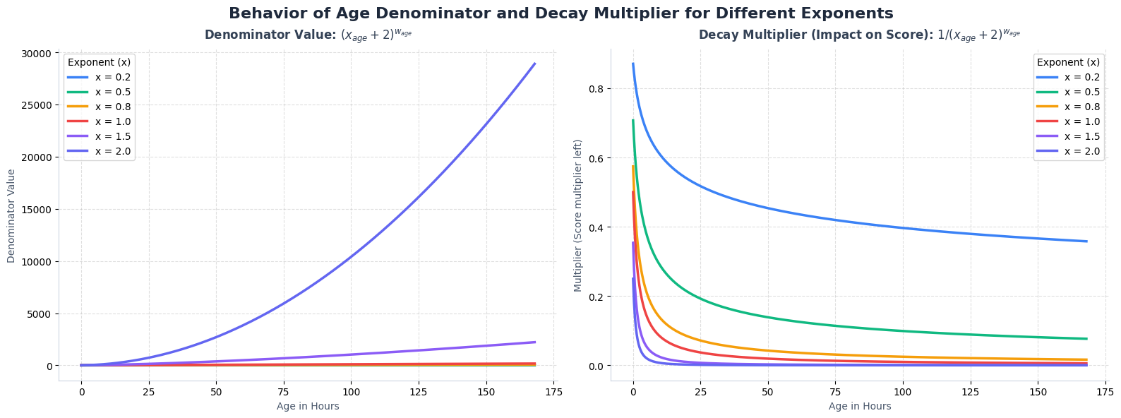
The is a non-zero value to ensure posts with zero votes and comments are ranked higher than posts with negative votes, while the is added to prevent division by zero (when ) and to dampen early decay (when ). There are a few problems with the current approach:
- Both and grow linearly, and can potentially blow up when there's an extremely viral post.
- Lack of other components that have influence on the relevance of a post, such as reputation of the author and the total vote counts.
- The hyperparameters are almost arbitrary, which might not be the optimal.
Clearly, we needed a revamp of the ranker and a smart, objective way to find the best hyperparameters.
Revamping the Ranker
To fix the first two issues, we proposed a refined ranker:
where the new post value, , is computed as:
The general intuition here is similar to the original ranker. The main difference is that we apply and (symmetric log: ) to positive-only and real-valued components before weighting them. This prevents viral posts from completely breaking the feed. We also introduced two new signals: the total vote count (to help weight the confidence of net votes) and the author's reputation (acting as a proxy for trustworthiness) to address the lack of context.
Solving the Optimal Weights Problem
Cool, now we have a refined ranker. But this is where the real challenge begins: how do we actually find the optimal hyperparameters?
First, let's define what "optimal" means for our forum. A great ranker should recommend posts that lead to clicks (high relevance) during a user's session. At the same time, we want to ensure users see a healthy mix of new posts (assuming new ones have been published). So, our goal is to maximize relevance while maintaining a certain level of freshness.
Formally, we define the objective as follows:
where is a browsing session, is the set of hyperparameters, is the number of clicks in session under , is the session's newness score, and is our minimum freshness threshold.
This is a great start. However, one limitation of this objective is that it does not account for the ranking order: if a user clicks four posts in a session, recommending those posts at the very top of the feed versus at the very bottom results in the same score. In practice, we want to present relevant posts as early as possible to capture user interest and prevent fatigue. To address this, we define the session score by discounting each click based on its position:
where is the set of clicked posts in session . This is essentially a simplified version of Discounted Cumulative Gain, where each clicked post has a binary relevance of 1.
LLM as Simulator
In an ideal world, we'd evaluate each hyperparameter set using real user interactions. But running A/B tests is pretty much impossible for us right now: our forum averages just 5-10 active users daily, meaning any live experiment would take forever and be incredibly noisy.
Instead, we decided to use Large Language Models (LLMs) to simulate user behavior. We prompt the LLM to model three basic actions:
- Click: The user finds a post interesting and clicks on it.
- Scroll: The user skips the current post but keeps scrolling.
- Quit: The user gets bored or tired and closes the tab.
Here is how we set up the simulation framework:
1. Simulating Sessions
Given some hyperparameters and all posts , we build a sequence of user sessions. Each session is defined by a login time . In that session, we only show posts created before , ranked in descending order by .
To determine , we group posts chronologically and trigger a login event every posts. We chose this over fixed time intervals because post frequency is highly non-uniform over time (it roughly follows a distribution). Since our forum has about 100 posts, we set to balance API costs with realistic timeline gaps.
This sequential setup is crucial. If we just showed all posts at once, we couldn't track whether a user had already seen a post in a previous session. That would reward bad hyperparameters that show the same posts over and over again.
2. Exhaustion Mechanism
A naive simulation where the LLM evaluates every single post in every session would require a quadratic number of API calls (). Since we're quite broke, we had to optimize this. We only call the LLM to evaluate new (unseen) posts, and model user fatigue through an exhaustion mechanism.
We set two parameters: a viewed count minimum and an exhaustion ratio . In any session, if the number of already-seen posts exceeds , and the ratio of seen posts to total posts encountered so far reaches , the simulation assumes the user is bored and terminates the session.
The intuition is that if the majority of the posts encountered in a session have already been seen, users are unlikely to keep scrolling, quickly becoming fatigued and exiting.
3. User Personas
To ensure the LLM responses are representative of our target users rather than general web users, we define three distinct student personas:
- The Hyper Achiever: The career-obsessed student who only cares about internships, competitive jobs, and academic queries, while ignoring social chatter.
- The Typical Student: A balanced student looking for campus life, study tips, and relatable career advice, actively avoiding toxic competitiveness and forum drama.
- The Lost Freshman: An overwhelmed first-year student trying to navigate logistics, make friends, and survive imposter syndrome, skipping advanced academic or career content.
4. Aggregating The Results
Finally, we average the simulated and across all sessions to compute the final objective score.
Pseudocode
def simulate_sessions_batch(all_posts, hyperparameters):
    # Sort posts chronologically (oldest first)
    posts = sort_by_date_ascending(all_posts)

    # Initialize results and user history for each persona
    results = {persona: {"clicks": 0, "views": 0, "discounted_clicks": 0.0} for persona in PERSONAS}
    viewed = {persona: set() for persona in PERSONAS}

    # Simulating Sessions: Trigger login events chronologically every N posts
    N = 10
    total_sessions = ceil(len(posts) / N)

    for session_idx in range(total_sessions):
        # Determine current login time (T_i)
        cutoff_index = min(len(posts), (session_idx + 1) * N) - 1
        T_i = posts[cutoff_index].created_at

        # Display only posts created before T_i, ranked by heuristic f(x; H)
        active_posts = filter_by_date(posts, before=T_i)
        ranked_posts = sort_by_score(active_posts, weights=hyperparameters)

        # Simulate each persona browsing the feed
        for persona in PERSONAS:
            clicks_count = 0
            views_count = 0
            seen_count = 0
            discounted_clicks_count = 0.0

            inputs_list = []
            valid_posts = []

            # 1. Exhaustion Mechanism & Duplicate Filtering BEFORE LLM calls
            for idx, post in enumerate(ranked_posts):
                if post.id in viewed[persona]:
                    seen_count += 1
                    # Fatigue check: terminate early if seen ratio/count exceeds limits
                    if seen_count >= DUP_COUNT_LIMIT and (seen_count / (idx + 1)) >= DUP_RATIO_LIMIT:
                        break
                    continue  # Skip evaluating duplicates

                if len(valid_posts) >= MAX_EVAL_POSTS:
                    break

                # Queue unseen post for batch evaluation
                inputs_list.append(prepare_llm_input(persona, post, rank=idx + 1))
                valid_posts.append(post)

            if not inputs_list:
                continue

            # 2. Call the LLM in batch (runs requests concurrently to optimize API speed)
            responses = query_llm_batch(inputs_list)

            # 3. Process the results sequentially to respect the 'quit' logic
            for idx, (post, decision) in enumerate(zip(valid_posts, responses)):
                # Mark post as viewed
                viewed[persona].add(post.id)

                if decision == "quit":
                    break

                views_count += 1
                if decision == "click":
                    # Calculate Discounted Clicks (Discounted Cumulative Gain)
                    rank = idx + 1
                    discounted_clicks_count += 1.0 / log2(rank + 1)
                    clicks_count += 1

            # Accumulate session counts
            results[persona]["discounted_clicks"] += discounted_clicks_count
            results[persona]["clicks"] += clicks_count
            results[persona]["views"] += views_count

    # 4. Aggregating The Results: Average metrics across all sessions
    for persona in PERSONAS:
        results[persona]["discounted_clicks"] /= total_sessions
        results[persona]["clicks"] /= total_sessions
        results[persona]["views"] /= total_sessions

    return results
Constrained Optimization
A straightforward way to solve this constrained optimization problem is through offline optimization. Under this approach, we would run simulations across a grid of hyperparameter configurations to generate training data, build two surrogate models to map any hyperparameter set to its expected click and newness metrics, and solve the Lagrangian using an offline solver.
However, the major limitation of this approach is its heavy dependence on the accuracy of the surrogate models. To train reliable models, we would need a large, representative dataset of simulations. This is highly impractical for us because a single simulation run can take a long time, making grid-based data generation prohibitively slow and expensive.
So, we opted for online optimization. Instead of guessing the whole parameter space upfront, we optimize in an active, closed loop. To do this efficiently without blowing through our API limits, we turned to Constrained Bayesian Optimization (BO).
To frame the problem, we need to define two components: the surrogate models and the acquisition function.
Surrogate Models
The job of our surrogate models is to estimate the clicks and newness functions, but more importantly, to quantify how unsure they are. We use these uncertainty estimates to guide our parameter choices in the loop. To stay sample-efficient, we train two independent Gaussian Processes (GPs), and . At any hyperparameter set , they give us a normal distribution of what they expect the clicks and newness to be:
where and is the mean and standard deviation of the normal distribution, respectively.
Acquisition Function
With our GP models in place, we need a way to actually choose the next parameters. This is where the acquisition function, , comes in. It scores any candidate by balancing how good we think it is with how unsure we are:
where is the expected improvement for the objective (clicks), and is the probability of feasibility (the probability that the newness constraint is satisfied). Formally, they are defined as:
where the Z-scores are computed as:
Here, is the maximum expected click rate observed so far among feasible hyperparameter configurations, and denote the standard normal cumulative distribution function (CDF) and probability density function (PDF), respectively.
Intuitively, balances exploitation (targeting configurations with high expected click rates ) and exploration (targeting areas with high uncertainty ). penalizes regions of the hyperparameter space that are likely to violate the minimum newness constraint. Multiplying the two terms yields a unified utility score that represents the overall potential of sampling next.
Putting It All Together
With these components defined, the complete Bayesian Optimization loop is structured as follows:
- Fit the surrogate models and on the training data (, , and ).
- Find the next hyperparameter candidate that maximizes the acquisition function using a solver.
- Run the simulation for and append the new observations to the training datasets.
- Repeat.
Results
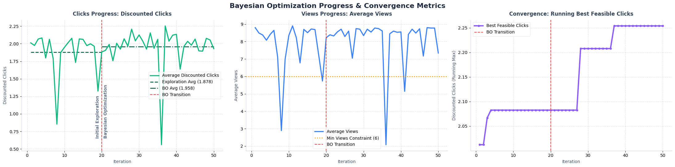
To evaluate the optimization process, we ran a total of 50 simulations. The first 20 iterations served as a pure exploration phase (sampling the parameter space uniformly), while the remaining 30 iterations were guided by the BO loop.
In terms of optimization progress, BO successfully maximized click rates, as indicated by a higher average click yield compared to the initial exploration phase. The overall headroom for improvement was relatively constrained, we believe this is due to the limited size and diversity of our dataset, as well as the rigid architecture of the heuristic ranker. Nevertheless, by the end of the optimization loop, we achieved an approximate 10% improvement over the best parameter configuration found during the pure exploration phase.
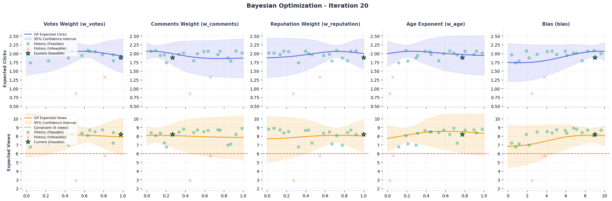
We can also observe how BO selects its next query candidate. As we know, BO balances exploitation and exploration while simultaneously satisfying the constraints. Visualizing the GP predictions for clicks and views at iteration 20 illustrates this behavior: the acquisition function prioritizes a candidate with a high potential click yield while avoiding regions likely to violate the view constraint.
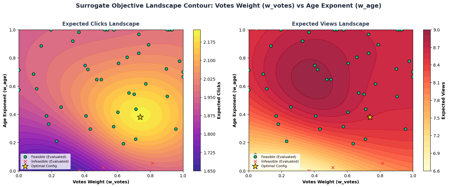
By fitting the GP model on all 50 observations, we can map the sensitivity of expected clicks and views to the two primary parameters: the age decay rate and the votes weight. As expected, a very low age decay rate tends to trigger constraint violations because old posts linger indefinitely on the feed. While a very high decay rate drives up views by constantly circulating fresh posts, it is sub-optimal for click yield because recency alone does not guarantee relevance. Ultimately, the optimization converges on a moderate decay rate for age paired with a high weight for votes.
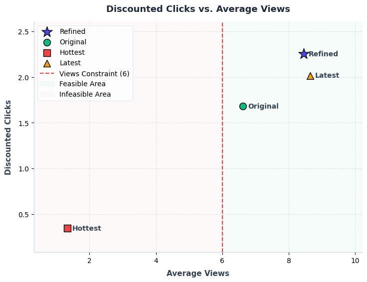
Finally, we evaluate the optimized weights against three baselines: the original heuristic (the legacy ranker currently serving the forum), hottest (sorting strictly by votes), and latest (sorting strictly by recency). Compared to the best-performing baseline (latest), our refined parameters yield an 11.87% improvement in clicks. More significantly, they deliver a 34.13% improvement over the original production ranker. As expected, the hottest baseline performs poorly because it ignores temporal decay, causing the feed to become stale and lose user engagement.
| Model | Discounted Clicks | Views | Improvement |
|---|---|---|---|
| refined | 2.254115 | 8.444444 | - |
| original | 1.680561 | 6.622222 | +34.13% |
| hottest | 0.348715 | 1.333333 | +546.41% |
| latest | 2.014915 | 8.644444 | +11.87% |
You can find the complete source code for this project on GitHub.
Final Thoughts
Since starting my job on the ETA & pricing team at Grab, I've run into a lot of constrained optimization models. They really sparked my interest, which is what ultimately inspired this project. It took me a while to actually get started, but I'm really glad I finally saw it through. I learned a ton about constrained optimization and had a blast building the optimization and simulation loop. Also, shout out to my guy Dong Yu for lending me his DeepSeek API key for the LLM simulations. Hope you learned something from this post, too!