I've always been curious about Reinforcement Learning (RL) ever since I first heard about it. The concept of an agent self-learning by interacting with its environment just sounded incredibly cool to me! A few years back, I built an RL agent to play snake game, but the core concepts remained vague and I didn't feel like I truly understood them. It wasn't until OxML, where I had the chance to hear about a lot of cool RL projects, that I decided to finally learn RL for real, this time starting from scratch.

So, I picked up Reinforcement Learning: An Introduction (the RL bible) and read through most of it, along with Grokking Deep Reinforcement Learning. (If you're interested, I've implemented some of the well-known Deep RL algorithms here.)

After working through both books, I wanted to put what I learned to the test. But I didn't know what I want to do until a month or two before starting this project, I came across an inspiring Clash Royale agent project. That pushed me to build an agent for a game of my own. What better choice than a game I used to spend hours playing (even tho I sucked at it)? So, I chose CS. And that's how it all started.

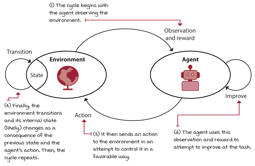
For those who aren't familiar with RL, here's a quick look at how the agent-environment cycle works:

The RL cycle, taken from Grokking Deep Reinforcement Learning.

The Counter Strike Agent

Since the main purpose of this project is educational, it is scoped to be manageable (and cheap, i.e., computationally feasible to train on my personal laptop because I'm broke). Essentially, the project aims to train a CS2 agent for Deathmatch, where the goal is simply to eliminate as many opponents as possible. To keep things simple, the agent is trained exclusively on the classic fy_snow map from CS 1.6 (chosen for its simple structure) and restricted to using only the AK-47. If you played old-school CS back in the day, you'd probably recognize this map:

fy_snow.

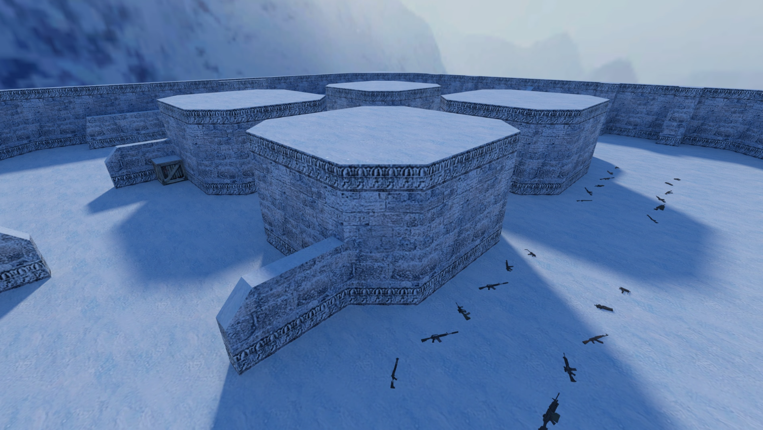
This map isn't directly available in CS2, but luckily, someone made a workshop version of it! So, I was able to get it running in CS2.

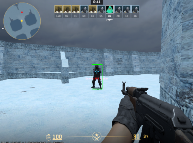
Since I am training and running inference on a personal laptop with an almost decade-old GPU, doing this in real time at normal game speed would cause severe input latency for the agent. For this reason, the game speed (host_timescale) is set to 0.5. To keep the computational workload light, the agent doesn't process raw visual pixels, instead, it operates on object bounding boxes. Thanks to the awesome open-source community, pre-trained models like Yolov5ForCSGO saved me from having to train (and painfully hand-label) a custom YOLO model.

Agent bounding boxes on fy_snow.

Building the Environment

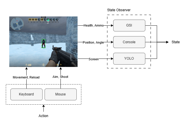
We have the game running on our laptop, and the resulting agent will most likely be running on a Python script. But how does the agent observe and interact with the game exactly? The answer is an environment, which acts as a bridge allowing the agent to observe states (e.g., coordinates, aiming angles, health) and execute actions (e.g., movement, aiming, firing).

Building this environment was tricky, but I managed to pull it off with a combination of hacks :P. The environment consists of two main components:

• State Observer: Responsible for gathering game observations across three different channels:
  • Game State Integration (GSI): Valve's official Game State Integration (GSI) API that extracts basic game stats like health, ammo, and kill count. Since GSI requires sv_cheats=1, the agent is restricted to private servers (which is sad because it means it's not possible to deploy the agent to online servers).
  • Console Commands (getpos): Because GSI doesn't expose both player coordinates and angles, I had to set up an infinite loop on a separate thread to send the getpos command to the in-game console to retrieve real-time position and orientation data.
  • YOLO: Finally, to detect enemy positions, I used a pre-trained YOLO model that parses game frames and outputs enemy bounding box coordinates.
• Action Handler: Manages agent inputs in real time. Keyboard movements and mouse movements / clicks use different components for control. The former uses pyautogui, while the latter uses low-level Windows API calls via Python's ctypes, which worked like a charm!

The environment.

Markov Decision Process

Now that we have the environment set up, let's formally frame this problem for RL, specifically as a Markov Decision Process (MDP), which is defined by the tuple $\mathcal{M} = (\mathcal{S}, \mathcal{A}, \mathcal{P}, \mathcal{R}, \gamma, \rho_0)$:

• State Space ($\mathcal{S}$): The state $s_t = [c_t, b_t, o_t]$ combines three elements:

  • $c_t$: Contextual stats including health, ammo, velocity, player coordinates, and aiming angles.
  • $b_t$: Bounding box coordinates ($x, y, w, h$) of the enemy detected by YOLO, where $x$ and $y$ are normalized w.r.t. the screen center. For simplicity and computational efficiency, we only use the bounding box of the primary target (the largest detected enemy bounding box).
  • $o_t$: A 2D occupancy grid giving the agent spatial awareness of the map.

• Action Space ($\mathcal{A}$): The action $a_t$ combines discrete and continuous controls:

  • $a_{\text{discrete}}$: Binary flags for shooting, reloading, and directional movement.
  • $a_{\text{continuous}}$: Continuous mouse rotation angle (yaw delta). Pitch delta was excluded to reduce learning complexity. For simplicity, the agent only controls horizontal aiming.

• Transition Dynamics ($\mathcal{P}$): $\mathcal{P}(s_{t+1} \mid s_t, a_t)$ represents the environment transitions governed by the CS2 game engine and physics.

• Reward Function ($\mathcal{R}$): A shaped multi-component reward function to guide learning:

  $$r_t = w_{\text{on}} \cdot R_{\text{on\_target}} + w_{\text{off}} \cdot R_{\text{off\_target}} + w_{\text{ammo}} \cdot R_{\text{ammo}} + w_{\text{health}} \cdot R_{\text{health}}$$

  Where:

  • $R_{\text{on\_target}} = +1$ when shooting while the crosshair is inside an enemy bounding box ($|\Delta x| \le \frac{w}{2} \land |\Delta y| \le \frac{h}{2}$) with ammo available. We use on-target shooting as the primary reward rather than kills, for reasons detailed in the next section.
  • $R_{\text{off\_target}} = -1$ when shooting with the crosshair outside target bounding boxes.
  • $R_{\text{ammo}} = -1$ when attempting to shoot with an empty magazine.
  • $R_{\text{health}}$ penalizes any loss in player health.

• Discount Factor ($\gamma$): Set to $0.95$ to balance immediate feedback with longer-term outcomes.

• Initial State Distribution ($\rho_0$): Defined by spawning (or respawning) at a random location on fy_snow with full health and a fresh magazine.

Bootstrapping the Agent

The problem with this MDP is that the reward is extremely sparse and the environment cannot be easily parallelized. If we were to let the agent learn from scratch by interacting with the environment with zero prior knowledge, it would be almost impossible to learn a decent policy. Given this limitation, we turn to Offline Reinforcement Learning, where the idea is to teach the agent instead of letting it learn from scratch, i.e., bootstrapping the RL policy with an existing dataset.

Since there is no readily available dataset for our defined MDP, I personally played around 150 episodes of gameplay on fy_snow while recording the transition tuples. This resulted in about 50,000 experience tuples.

During data analysis, we observed that a portion of kill frames in the demonstration dataset lacked bounding boxes, likely due to accuracy limitations of the object detection model. To avoid introducing noise into policy learning (such as rewarding shooting without a bounding box present), we excluded raw kills from the reward function.

Among the spectrum of offline RL methods, we chose Implicit Q Learning because the idea behind it is simple and elegant. Best of all, it can easily be extended to online RL, allowing the agent to continue learning on its own after initial bootstrapping. But let's not get ahead of ourselves! First, let's talk about how IQL works.

Implicit Q Learning

To learn the optimal state-action value function $Q_{\pi^*}$, standard tabular Q-learning iteratively updates $Q(s, a)$ via:

In deep RL, we can adopt a similar principle to update our Q-network by minimizing the temporal-difference (TD) loss:

However, in an offline setting, evaluating $\max_{a'} Q(s', a')$ poses a major challenge: it makes out-of-distribution queries for actions $a'$ that were rarely or never seen in the dataset $\mathcal{D}$, leading to severe overestimation of Q-values.

Implicit Q-Learning (IQL) addresses this by approximating $\max_{a'} Q(s', a')$ using expectile regression to learn a state-value function $V_{\psi}(s')$, thereby completely avoiding queries to out-of-distribution actions:

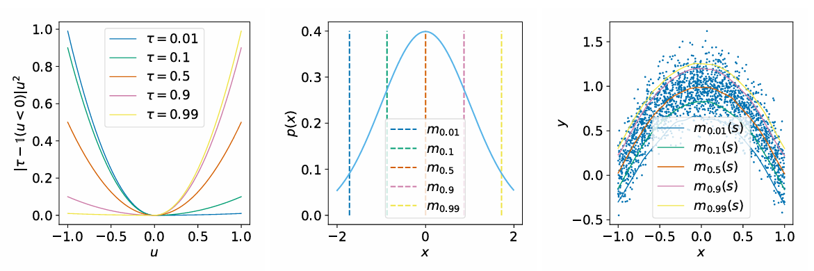
where $V_{\psi}(s)$ is fitted using the expectile loss:

Here, $L^\tau_2(u) = |\tau - \mathbf{1}(u < 0)| u^2$ is the asymmetric squared loss, where $u = Q_{\theta}(s, a) - V_{\psi}(s)$. The parameter $\tau \in (0, 1)$ controls how closely $V_{\psi}$ approximates the maximum value versus the mean. Below is a helpful visualization showing how expectile regression behaves for different values of $\tau$:

Left: loss value for different tau. Center: expectiles of a normal distribution. Right: expectile regression of a two dimensional random variable.

While learning $Q_{\theta}$ and $V_{\psi}$ yields the value functions, it does not directly give us an executable policy. To extract the policy $\pi_{\phi}$, IQL uses Advantage-Weighted Regression (AWR) to fit the policy via weighted log-likelihood:

Here, $Q_{\theta}(s,a) - V_{\psi}(s)$ represents the estimated advantage of action $a$, where the inverse temperature parameter $\beta \ge 0$ controls policy greediness: larger values exponentially favor high-advantage actions toward the optimal policy, while $\beta \to 0$ reduces the objective to standard Behavioral Cloning (BC). This can be thought as REINFORCE-style score function updates, but with an exponentiated advantage weight to make it work offline.

Network Architecture

Due to computational constraints (and the fact that I am broke), I adopted a lightweight architecture combining MLPs with convolutional blocks to process the 2D occupancy grid and estimate $Q_{\theta}$, $V_{\psi}$, and $\pi_{\phi}$.

Network Architecture.

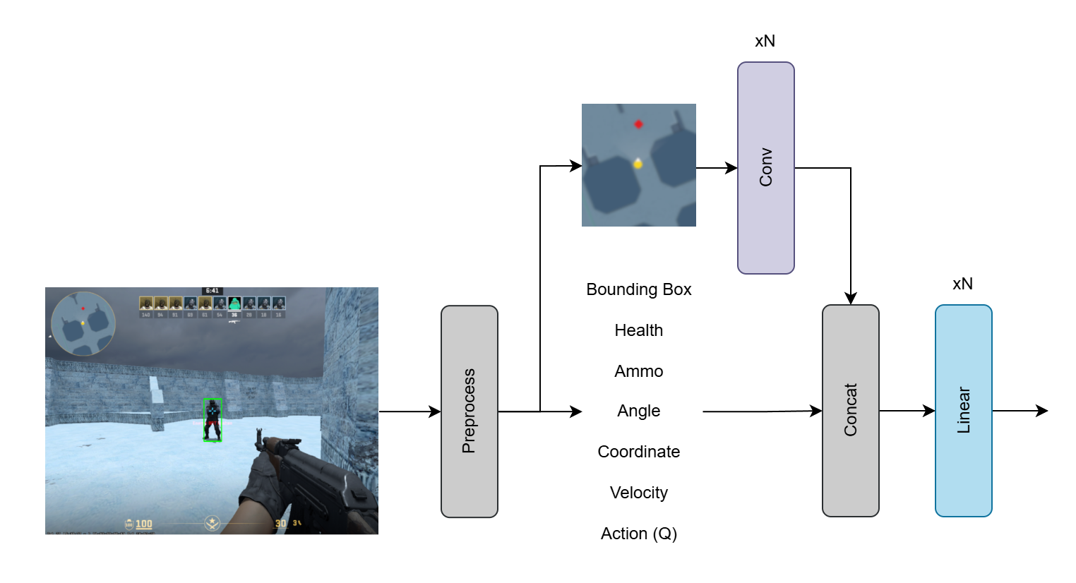
All three networks use the same backbone architecture. The primary differences lie in their final output heads and training objectives.

For the policy network $\pi_{\phi}$, the output consists of parameters for action-specific probability distributions. For discrete actions (e.g., shooting, reloading, and directional movement), the network outputs logits parameterizing a Bernoulli distribution, and for continuous actions (i.e., horizontal mouse yaw delta), the network outputs the mean $\mu$ and standard deviation $\sigma$ of a Gaussian distribution.

Stratified Sampling

As mentioned earlier, transitions with positive rewards are far sparser than those with zero or negative rewards:

Transition distribution across reward segments (only ~11% contain positive rewards).

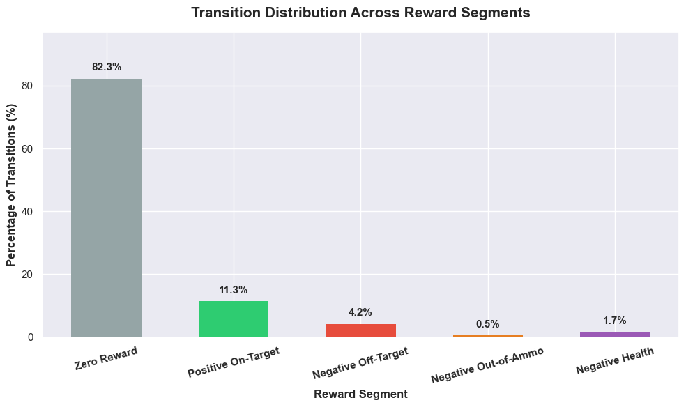
To address this imbalance, we structured the sampling distribution $\mathcal{D}$ to consist of 35% random transitions, 30% on-target shots ($R_{\text{on\_target}} > 0$), 15% off-target shot penalties ($R_{\text{off\_target}} < 0$), and 20% transitions from the 10 timesteps leading up to a kill. This stratified sampling scheme ensures the model effectively learns what is desirable (on-target shooting), how to achieve it (trajectories leading up to kills), what to avoid (off-target shots), and how to navigate on average (random baseline transitions).

Taking the Agent Live

Offline IQL alone can yield a surprisingly capable agent, one that behaves similarly to the human demonstrator while effectively distinguishing between good and bad actions. Given a sufficiently large and diverse dataset, an offline agent can perform on par with humans. However, we shouldn't stop here for two key reasons: (1) our demonstrations are relatively limited and may not cover all edge cases, leaving the agent uncertain in unfamiliar situations, and (2) we want the agent to discover strategies that surpass human demonstration. Therefore, the next natural step is to transition to online RL, allowing the agent to directly interact with, explore, and exploit the environment.

To bridge the gap from offline RL to online RL without causing policy collapse, we introduce a few components to our setup.

Replay Buffer

In the offline phase, our dataset $\mathcal{D}$ consisted purely of demonstration data. To enable online learning, we need a mechanism to continuously collect and store real-time experiences from the agent's interactions.

We accomplish this using a fixed-size replay buffer capable of storing up to $N$ transition tuples. To prioritize fresh and recent experiences, the buffer retains only the latest $N$ transitions in a queue-like structure (FIFO).

We now have two distinct data sources: offline demonstrations and live online interactions. Moving forward, we denote the offline dataset as $\mathcal{D}_{\text{off}}$ and the online replay buffer as $\mathcal{D}_{\text{on}}$.

Dynamic Data Mixing

Having two distinct data sources, $\mathcal{D}_{\text{off}}$ and $\mathcal{D}_{\text{on}}$, also means that we need a way to sample them effectively. We do this by dynamically increasing the proportion of online samples across a number of episodes, which we call warm-up epochs ($N_{\text{warmup}}$), until reaching an upper bound $U$, instead of fully replacing offline data with online data.

Formally, at epoch $i$, we denote $P_{\text{on}}$ and $P_{\text{off}}$ as the proportion of online and offline samples used in the batch, respectively:

This allows the agent to learn more efficiently because the distribution doesn't suffer from a sudden shift, but rather a gradual one that RL is good at adapting to. We don't fully replace offline data because we believe there is still value in human demonstrations, as they tend to be more accurate and help prevent catastrophic forgetting in the model.

Online Exploration

When the agent is interacting with the environment, we can let the agent takes a deterministic set of actions that agent thinks its the best. However, the issue with this is that, we're limitting the interaction, or the experiences to be collected to train the agent limited to what it already think its good, hence, it has very little exploration.

Fortunately, because the policy network outputs probability distributions, we can sample actions stochastically to naturally incorporate exploration into the agent's online interactions:

Putting Everything Together

To tie all these components together, from multi-channel state observation and real-time input handling to hybrid offline/online IQL updates, here is the end-to-end architecture of our CS2 RL agent system:

Overall system architecture of the CS2 RL agent.

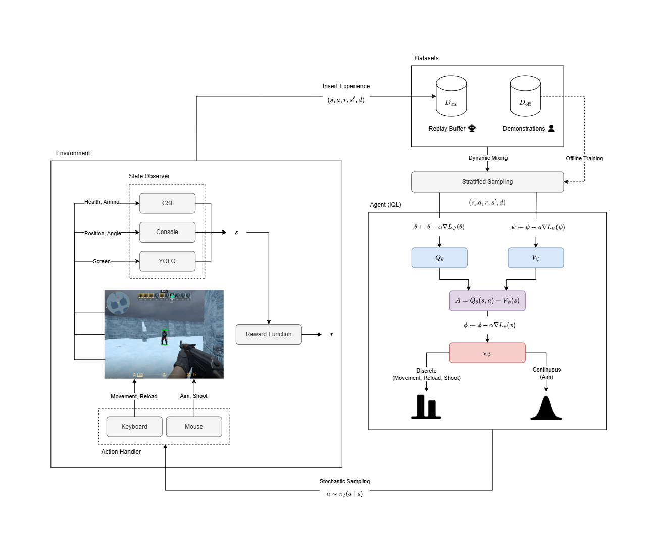
At a high level, the system operates across three main interconnected modules:

• Environment Loop: The State Observer gathers game state $s$ across GSI, developer console, and YOLO bounding boxes. Actions sampled stochastically $a \sim \pi_\phi(a|s)$ are sent to the Action Handler to execute simulated keyboard and mouse inputs.
• Data Pipeline: Environment transitions $(s, a, r, s', d)$ stream into the online replay buffer $\mathcal{D}_{\text{on}}$. During training, transitions are dynamically mixed with human demonstrations $\mathcal{D}_{\text{off}}$ and filtered through stratified sampling to tackle reward sparsity.
• Agent Optimization: The agent fits $V_\psi$ and $Q_\theta$, computes the advantage $A = Q_\theta(s, a) - V_\psi(s)$, and uses Advantage-Weighted Regression (AWR) to update the policy $\pi_\phi$.

Results & Evaluation

Enough said about the methodology, let's dive into the results now and see how well (or poorly) the proposed approach performed!

First, we examine the numerical results from offline and online training. Next, we evaluate the agent qualitatively across several key behaviors it was trained to learn. Finally, we look at some gameplay clips of the final model in action.

From Offline Bootstrapping to Online Fine-Tuning

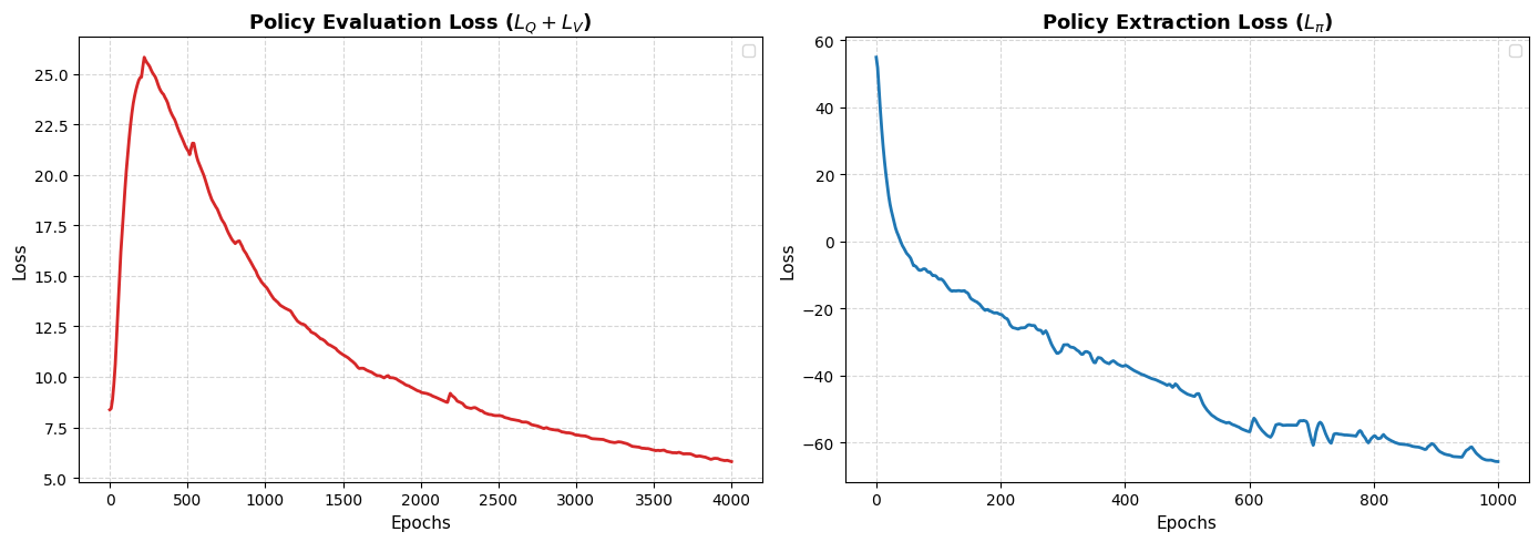
For offline training, we set the policy evaluation phase (training the $Q$ and $V$ networks) to 4,000 epochs and the policy extraction phase to 1,000 epochs. Neither network fully converged within this budget, however, from prior experiments, we didn't observe noticeable performance gains with additional epochs. Stopping early also allowed for faster iteration while training multiple model variants in parallel. In total, offline training took about 1-2 hours to complete.

Notice that during policy evaluation, the loss initially spikes before steadily decreasing. This is expected in Deep RL when training against a moving target, especially early on, when the model's predictions carry high uncertainty and incur large penalties. Around epoch 400, the loss begins to drop consistently.

Offline training curves: Policy evaluation loss (left) and policy extraction loss (right).

When the offline model was tested live in the environment, it fell apart pretty quickly. This was expected because the demonstration dataset was small and couldn't cover every edge case (as shown in the next section). To fix this, we put the model directly into the online RL loop, allowing it to interact, explore, and discover better strategies on its own.

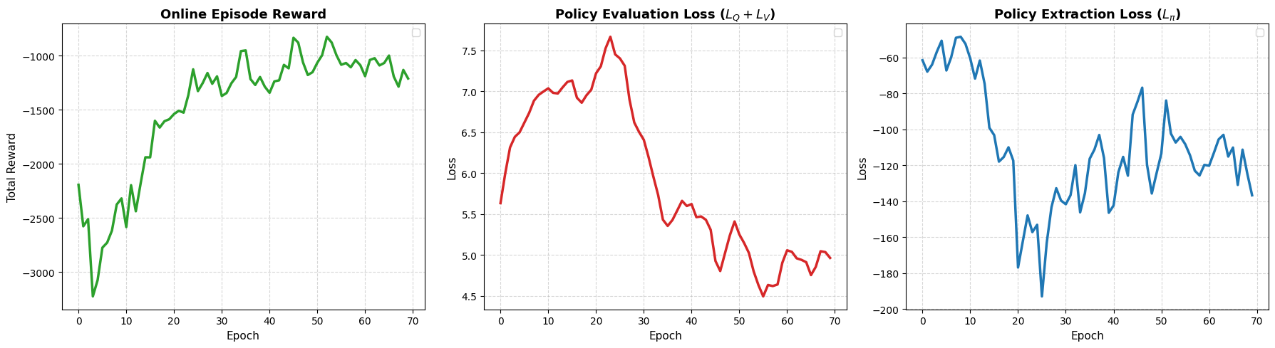
For online training, we set the total duration to 70 epochs. In each epoch, the agent collects 10 episodes of gameplay (each lasting up to 500 steps). A single epoch takes roughly 30 minutes, meaning the full 70-epoch run took nearly 1–2 days to complete. We set the warm-up period to 20 epochs and the upper bound $U = 0.7$, meaning the agent linearly scales its proportion of online experience over the first 20 epochs until online data makes up 70% of each training batch.

The offline model's struggle to generalize is clear in the early online epochs, where initial rewards take a heavy hit. But as online training progresses, performance improves dramatically: average episode returns climb from around -2500 up to -800 at its peak before stabilizing.

Online training curves. Left: episode returns. Middle and Right: policy losses.

Emergent Behaviors & Policy Analysis

Quantitative results show that online training yields significant improvements. In this section, we take a qualitative look at specific agent behaviors to better understand what it actually learned.

Firing Behavior Across Different Scenarios

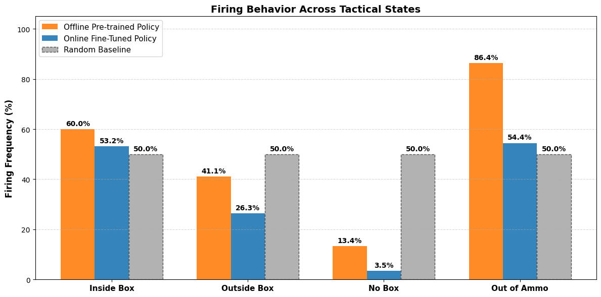
The agent's primary objective is to fire only when its crosshair overlaps with an enemy bounding box. Firing into thin air incurs a penalty, while attempting to shoot with an empty magazine incurs an even heavier penalty. In the comparison below, the offline agent frequently shoots when the crosshair is off-target, when no enemies are present, or when it runs out of ammo, largely because these negative scenarios were sparse in the demonstration data. Once fine-tuned online, the agent successfully learned to suppress firing in all three undesirable scenarios.

Firing behavior across different scenarios: offline agent vs. online fine-tuned agent.

Target Size vs. Firing Probability

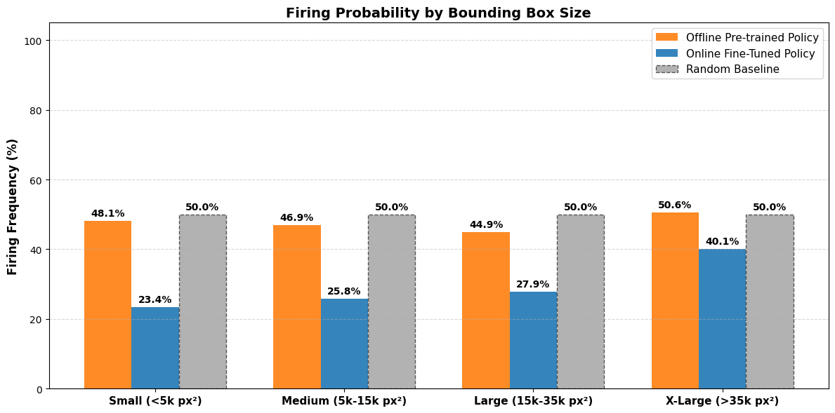
An interesting pattern emerged when looking at firing probability relative to target bounding box size. The offline agent attempts to shoot with high frequency regardless of target size. In contrast, the online fine-tuned agent learned that firing at small target boxes (distant enemies) carries a higher risk of missing, so it keeps its firing probability low (< 30%) at distance, reserving high firing probabilities for close-range engagements with larger bounding boxes.

Firing probability by target bounding box size.

Movement Speed During Engagements

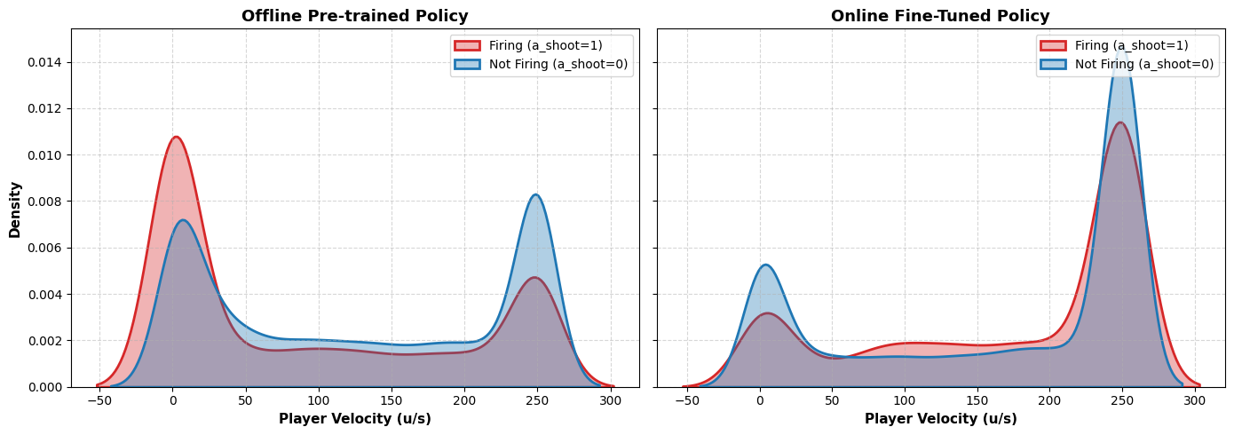
Firing while moving at high speeds causes severe recoil spread, sending bullets flying in every direction. Ideally, a skilled agent should decelerate to lower its velocity before firing. Interestingly, the online fine-tuned agent failed to pick up this nuance, exhibiting a velocity distribution peaked near maximum speed. Surprisingly, the offline agent captured low-velocity firing behavior much better, shown by a pronounced peak at near-zero velocity.

Distribution of player velocity while firing.

Target Tracking & Mouse Adjustments

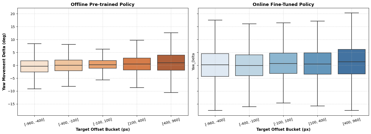
To land shots effectively, an agent must rapidly align its crosshair toward enemies. We visualized this by plotting horizontal target offset (how far an enemy bounding box is from screen center) against the agent's executed mouse yaw delta. An ideal aiming policy should exhibit a strong proportional relationship where larger target offsets should trigger larger yaw adjustments. Neither agent mastered this relationship cleanly, though both showed a mild positive correlation where larger offsets led to slightly larger mouse corrections.

Horizontal target offset distance vs. mouse yaw delta.

Spatial Perception & Pathfinding

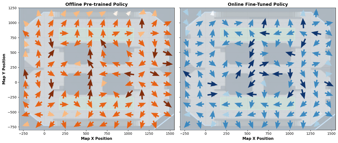
The agent relies entirely on raw player coordinates and a 2D occupancy grid for spatial awareness. To evaluate how well it navigates fy_snow, we plotted vector fields for both policies, where arrow direction represents movement direction and arrow size/intensity indicates visitation frequency.

Both models display dark vector trails through the center of the map, which makes intuitive sense, as that's where most engagements occur. The online agent shows much higher visitation density in these combat zones due to its extended exploration. Additionally, movement vectors form coherent pathways rather than random jitter.

Spatial vector fields showing agent movement direction and visitation frequency across fy_snow.

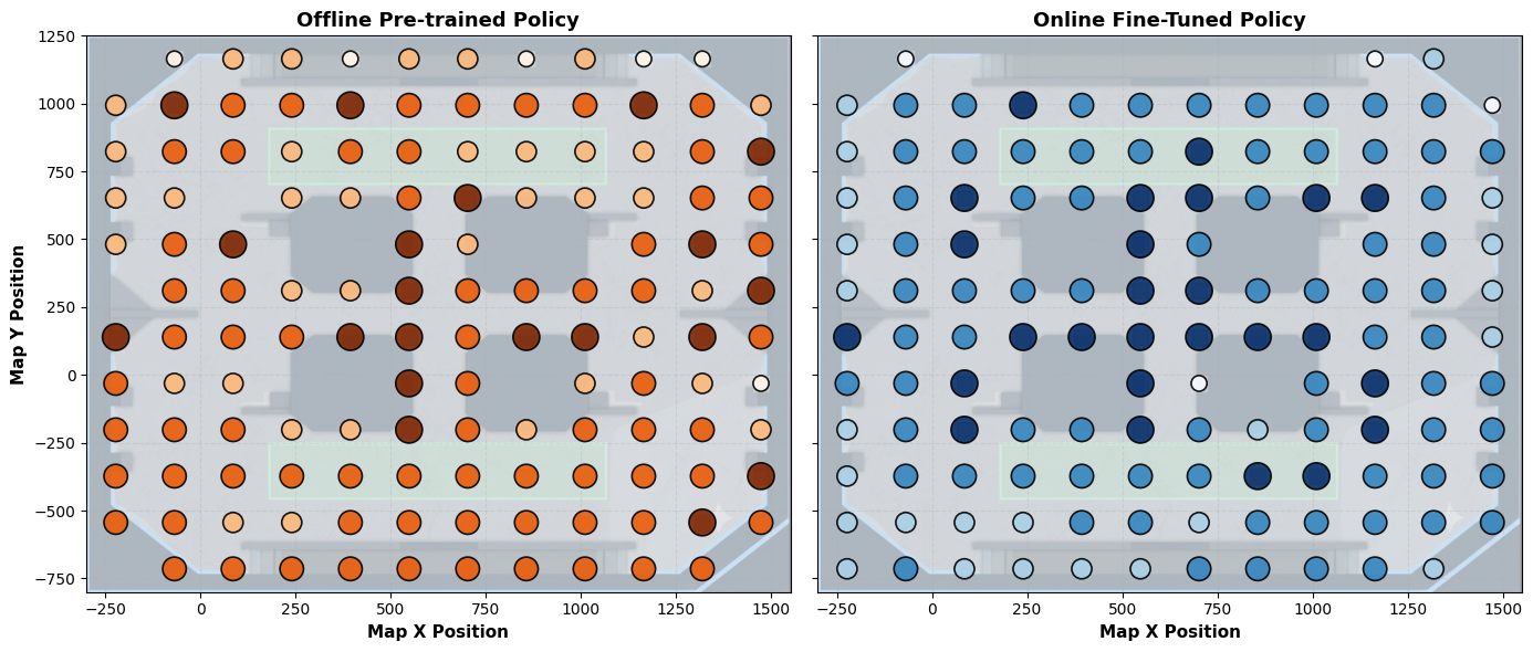
Cross-referencing this with a heatmap of kill intensity, we see that high-density combat zones align closely with the agent's heavy navigation paths.

Heatmap of kill density across the map.

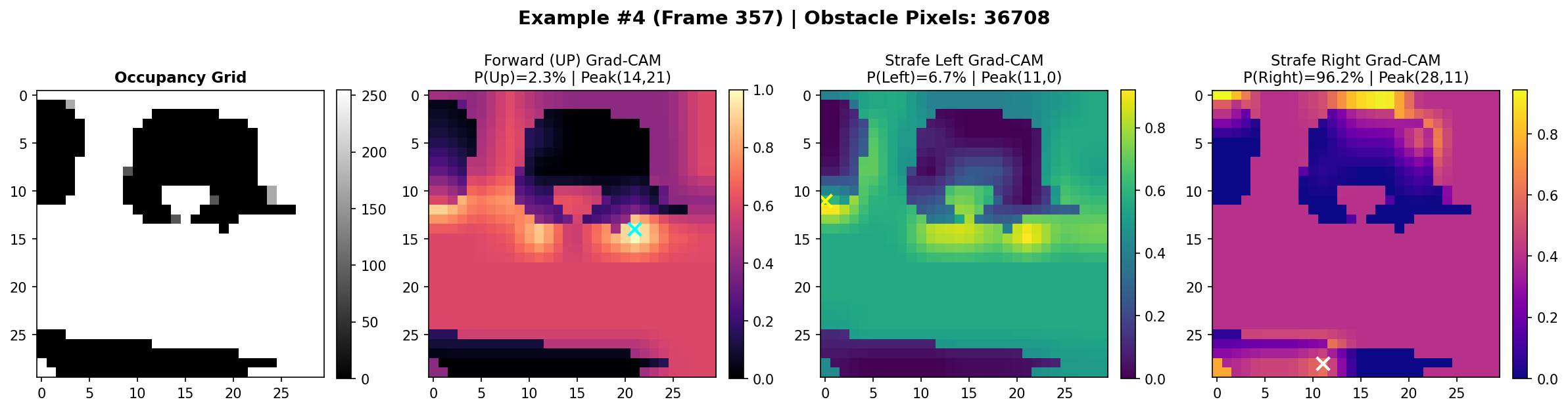
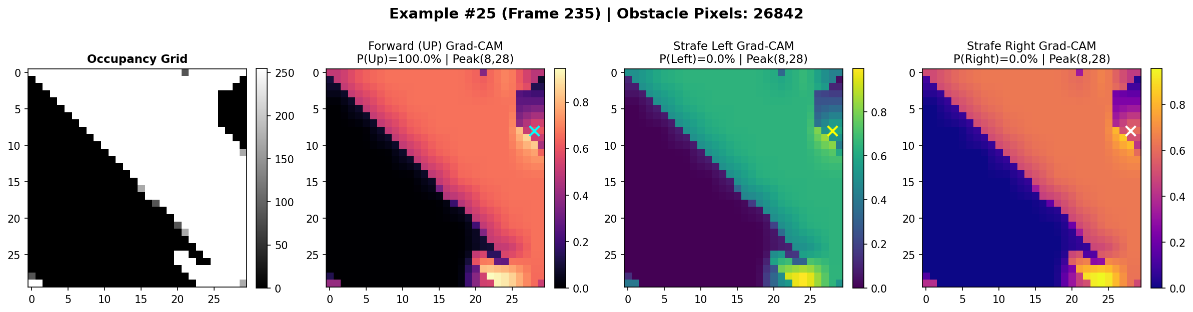
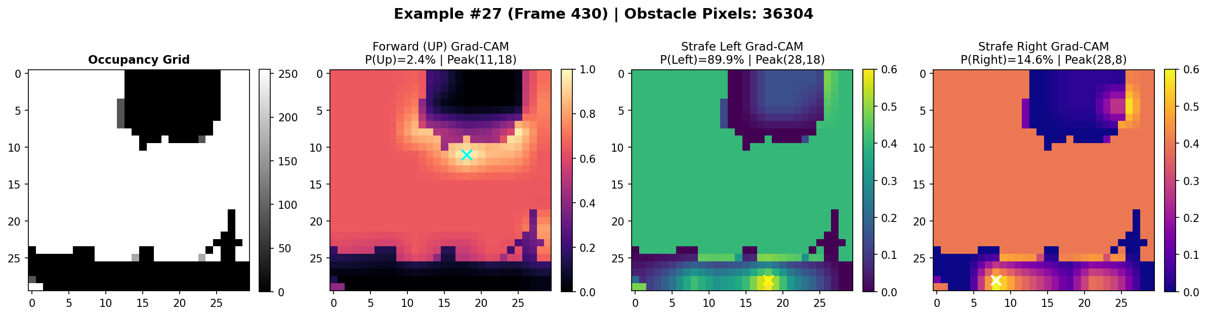
To understand how the agent uses its occupancy grid for obstacle avoidance, we applied Grad-CAM to inspect its movement decisions in several scenarios. In the first scenario, when faced with a large block directly ahead, the agent's forward movement probability drops significantly where Grad-CAM highlights strong network activation around the obstacle boundaries. In the second scenario, with clear space ahead, forward movement probability remains high with minimal blocking activations. In the third scenario, another obstacle directly ahead similarly triggers obstacle-focused activations and suppresses forward movement.

Grad-CAM visualizations highlighting occupancy grid regions that influence movement decisions.

Agent in Action

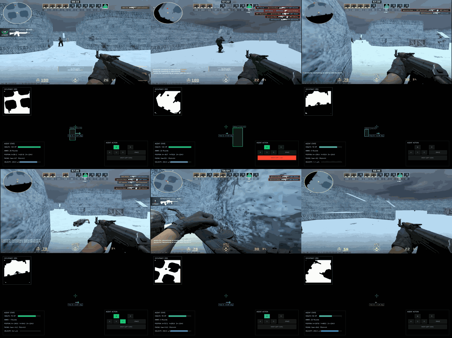
Finally, let's look at a demonstration of the resulting agent in action. The top view shows the actual in-game footage, while the bottom view displays what the agent perceives and how its policy reacts in real time. Overall, the agent demonstrates reasonable navigation around fy_snow and consistently opens fire when an enemy enters its field of view.

Agent gameplay demonstration. Top: raw CS2 footage. Bottom: agent perception and action output.

Conclusion

And that's all I've got for y'all! I hope you learned something useful from this write-up. The agent certainly won't be going pro anytime soon, but I believe with a bit more hyperparameter tuning (fine-tuning reward weights, expanding network capacity, and training for more epochs), its performance could improve significantly. Still, the main goal of this project was to build and understand a full Deep RL pipeline for CS from scratch, and I'd say we succeeded on that front!

The complete source code, pre-trained model artifacts, and datasets are open-sourced and available on GitHub. Feel free to check out the repository, try running the agent yourself!

Final Thoughts

From start to finish, this project took about 3–4 months to complete, with a 1–2 month break in between due to other commitments (~1 month spent brainstorming and building the offline/online training pipelines, and another month running a crazy number of ablations and experiments). I'm super glad I finally found the time to push it across the finish line. Even though the agent's gameplay is far from great, building every component from scratch was an awesome learning experience.

P.S. On a personal note, I'm really grateful I picked up RL before my MLE interviews at Grab, I genuinely believe it was one of the main reasons I landed the job!